NEO_AKSA

YOLO also know as You Only Look Once. Not like R-CNN, YOLO uses single CNN to do the object detection as well as localization which makes it super faster than R-CNN with only losing a little accuracy. From 2016 to 2018, YOLO has been imporved from v1 to v3. In this article, I will use a simple way to explain how YOLO works.

What tasks we need to solve in object detection problem?

Yolo use the same method as human to detect the object. There are three major steps: 1. is it an object? 2. what object is it? 3. where is the position and size of this object. BUT! Through CNN, YOLO can do these three things all together.

How YOLO solve this problem?

First, Let’s introduce Grid Cell in YOLO. The whole input image is divided into grid. Each grid cell predicts only one objects with fixed boundary boxes( say #B). For each boundary box has its own box confidence score to reflet the possibility of object. For each grid cell it predicts C conditional class probabilities( one per class). so that we will get
predictions. Here 5 means central location(x,y), size( h,w) and confidence score of each boundary box.

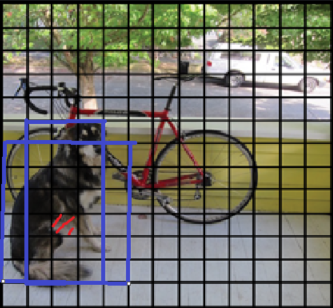
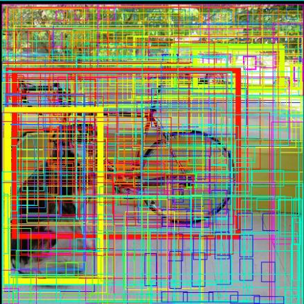
Then you will find so many boundary box from output. How we choose of them? Here we need to do Non-max suppression. The step is as blew:

1. discard all boxes with box confidence less then a threshold. ( say 0.65)
2. While there are any renaming box(overlapping):
   1. pick the box with the largest confidence that as a prediction
   2. discard any remaining boxes with IoU(intersection over union: you can see it as overlap size between two boundary box) greater than a threshold(say 0.5)

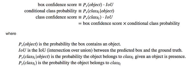
After Non-max suppression, we need to calculate class confidence score , which equals to box confidence score * conditional class probability. Finally, we get the object with probability and its localization. (see Figure 1)

YOLO Network Design

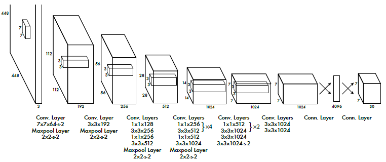
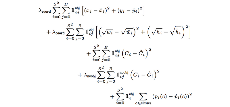
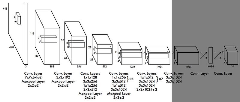
Let’s see how YOLO v1 looks like. Input = 448*448 image, output = . There are 24 convolutional layers followed by 2 full connected layer for localization. It use sum-squared error between the predictions and ground truth to calculate loss which is consist of classification loss, localization loss and confidence loss.

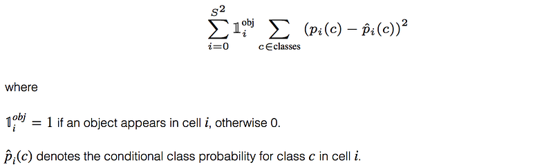
Classification loss:

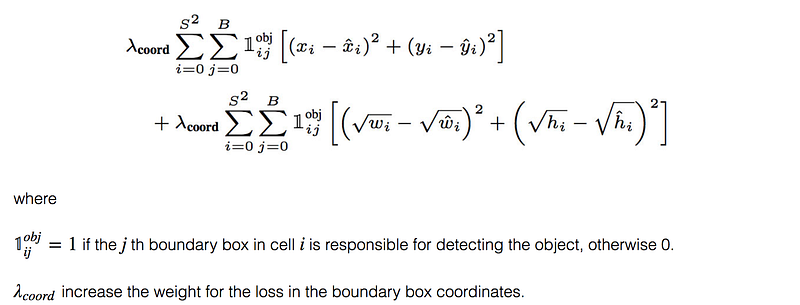
Localization loss:

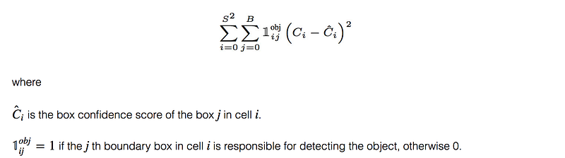
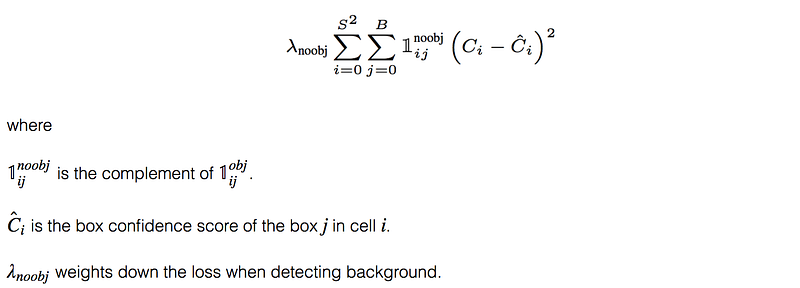
Confidence loss:

The final loss add three components together.

YOLO V2

YOLO v2 improves accuracy compared with YOLO v1.

1. Add batch normalization on all of the convolutional layers. It get more than 2% improvement in accuracy.
2. High-resolution classifier. First fine tune the classification network at the full resolution for 10 epochs on IMageNet. This gives network time to adjust tis filters to work better on higher resolution input.
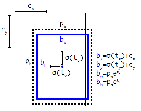
3. Convolutional with Anchor Boxes. YOLO v1 can only predicts 98 boxes per images and it makes arbitrary guesses on the boundary boxes which leads to bad generalization, but with anchor boxes, YOLO v2 predicts more than a thousand. Then it use dimension cluster and direct location prediction to get the boundary box.
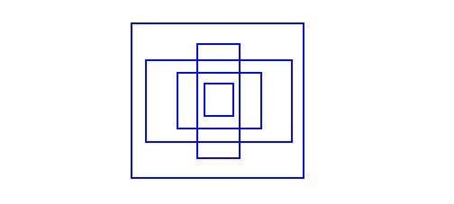
4. Dimension Cluster. use K-mean to get the boundary boxes patterns. Figure 5 might be the most common boundary boxes in spec dataset.

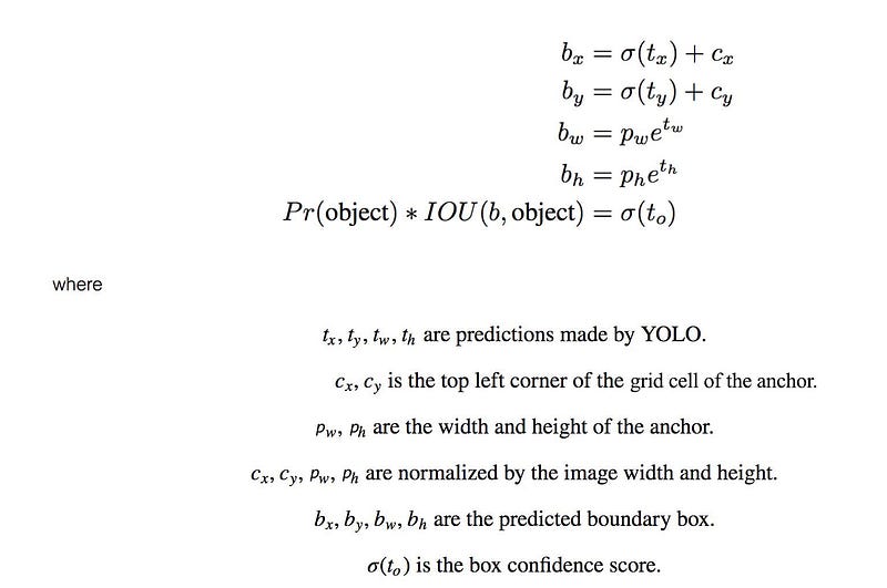
5. Direct location prediction. Since we use anchor boxes, we have to predict on the offsets to these anchors.

6. Multi-Scale Training. Every 10 batches, YOLOv2 randomly selects another image size to train the model. This acts as data augmentation and forces the network to predict well for different input image dimension and scale. 

YOLO v3

1. Detection at three scales. YOLOv3 predicts boxes at 3 different scales. Then features are extracted from each scale by using a method similar to that of feature pyramid networks
2. Bounding box predictions. YOLO v3 predicts the object score using logistic regression.
3. Class prediction. Use independent logistic classifiers instead of softmax. This is done to make the classification multi-able classification.

Reference:

YOLOv1 : https://arxiv.org/abs/1506.02640

YOLOv2 : https://pjreddie.com/media/files/papers/YOLO9000.pdf

YOLOv3 : https://pjreddie.com/media/files/papers/YOLOv3.pdf